Missing data mechanisms

Last updated on Jan 9, 2024 15 min read

In research, missing data occur when a data value is unavailable. Many empirical studies encounter missing data. Missing data can occur in many stages of research due to many different causes in many different forms. When invited respondents do not participate in the study there is non-response. It is also possible that for some particpants there are missing values in measured variables tahta are used as a predictor, covariate or outcome, i.e. intermittend missing data. When participants in a longitudinal study do not show up at one or more repeated measurement occasions, the missing data are often referred to as drop-out or loss to follow up.

Each type of missing data may have different reasons, and also different implication for the methods to deal with the missing data. To get more insight in the missing data problem, the reasons for missing data are differentiated in several missing data mechanisms. These mechanisms describe the underlying cause of missing data and were first described by Rubin (1976). Rubin distinguished three missing data mechanisms: missing completely at random (MCAR), missing at random (MAR), and missing not at random (MNAR). These missing data mechanisms are important since they are assumptions for the missing data methods. It must be noted that the missing data mechanisms are not characteristics of an entire data set, but the mechanisms are merely assumptions which apply to specific analyses methods.

Missing completely at random (MCAR)

Missing data are MCAR when the probability of missing data on a variable is unrelated to any other measured variable and is unrelated to the variable with missing values itself. In other words the missingness on the variable is completely unsystematic. For example questionnaire responses get lost in the mail.

Table 1: Description of fully observed data
	vars	n	mean	sd	median	trimmed	mad	min	max	range	skew	kurtosis	se
X1	1	1000	0.00	2.21	0.07	0.02	2.25	-7.42	6.69	14.11	-0.13	-0.13	0.07
X2	2	1000	0.09	2.26	0.14	0.12	2.24	-6.73	6.58	13.31	-0.12	-0.15	0.07
X3	3	1000	-0.03	2.25	0.02	-0.04	2.27	-7.27	6.54	13.81	0.00	-0.22	0.07

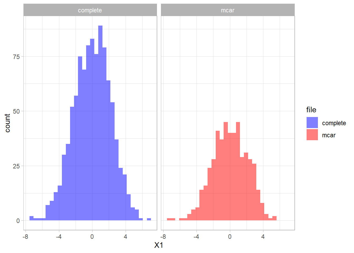
When we create MCAR data for 50% of the subject in variable X1 we see that the statistics for variable X1 have not changed much:

set.seed(8965)
mcar <- MCAR(x, alpha = 0.5, pattern = matrix(c(0,1,1), nrow = 1))

Table 2: Description of MCAR data - 50%
	vars	n	mean	sd	median	trimmed	mad	min	max	range	skew	kurtosis	se
X1	1	490	0.01	2.10	0.02	0.04	2.14	-7.38	5.58	12.96	-0.18	-0.10	0.09
X2	2	1000	0.09	2.26	0.14	0.12	2.24	-6.73	6.58	13.31	-0.12	-0.15	0.07
X3	3	1000	-0.03	2.25	0.02	-0.04	2.27	-7.27	6.54	13.81	0.00	-0.22	0.07

The distribution of the fully observed version of the variable is depicted in blue and the remaining data due to missings is red. As a result the missing part of the data are the blue parts of the graph.

We can create a missing data indicator variable R1 to explore differences between the subjects with missing data and the subjects without missing data.

mcar <- mcar %>% mutate(R1 = is.na(X1))

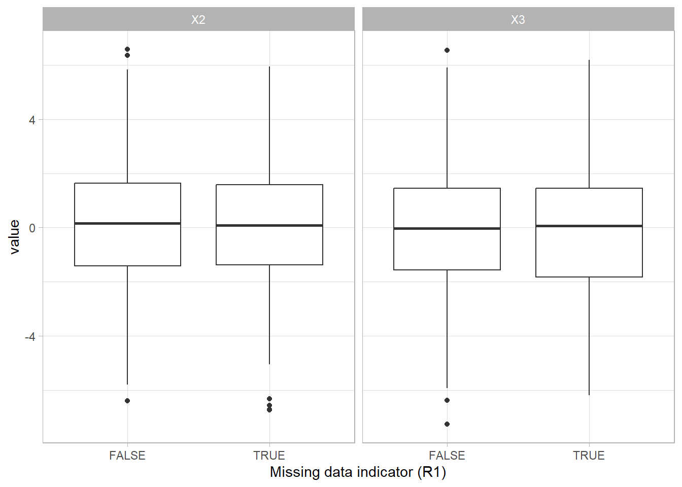
Missing completely at random (MCAR) is the only missing data mechanism that can actually be verified. This assumption can be tested by separating the missing and the complete cases and examine the group characteristics. If characteristics are not equal for both groups, the MCAR assumption does not hold.

Missing at random (MAR)

Missing data are missing at random (MAR) when the probability of missing data on a variable is related to some other measured variable in the model, but not to the value of the variable with missing values itself. For example, only younger people have missing values for IQ. In that case the probability of missing data on IQ is related to age. The assumption that the mechanism is MAR, can unfortunately not be confirmed, because it cannot be tested if the probability of missing data on a variable is solely a function of other measured variables. It is recommended to incorporate correlates of missingness into the missing data handling procedure to diminish bias and improve the chances of satisfying the MAR assumption.

Table 3: Description of fully observed data
	vars	n	mean	sd	median	trimmed	mad	min	max	range	skew	kurtosis	se
X1	1	1000	0.00	2.21	0.07	0.02	2.25	-7.42	6.69	14.11	-0.13	-0.13	0.07
X2	2	1000	0.09	2.26	0.14	0.12	2.24	-6.73	6.58	13.31	-0.12	-0.15	0.07
X3	3	1000	-0.03	2.25	0.02	-0.04	2.27	-7.27	6.54	13.81	0.00	-0.22	0.07

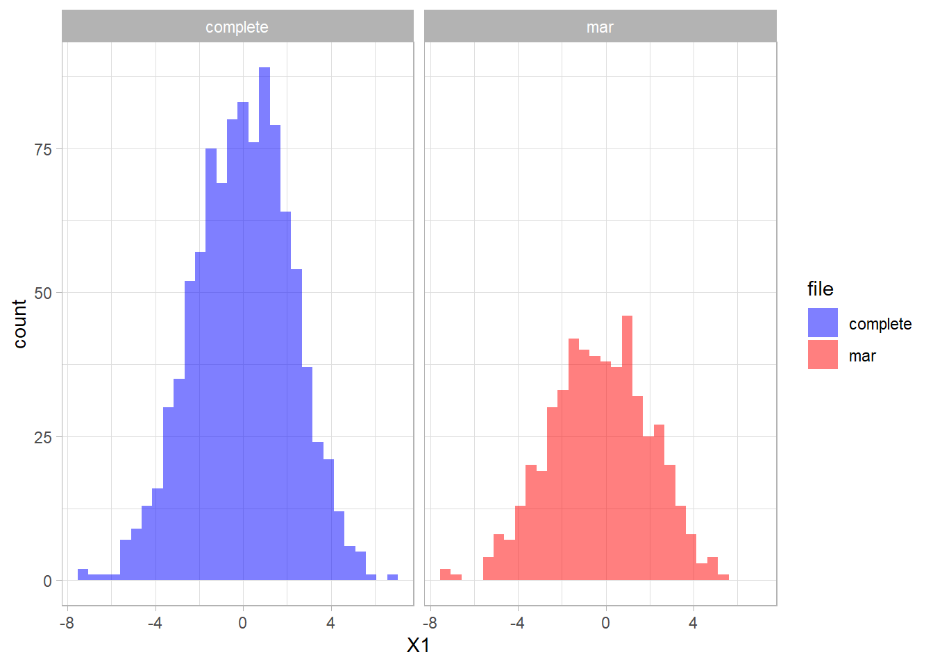
When we create MAR data for 50% of the subject in variable X1 we see that the statistics for variable X1 have changed:

set.seed(4665)
mar <- MAR(x, alpha = 0.5, pattern = matrix(c(0,1,1), nrow = 1))

Table 4: Description of MAR data - 50%
	vars	n	mean	sd	median	trimmed	mad	min	max	range	skew	kurtosis	se
X1	1	512	-0.28	2.25	-0.27	-0.26	2.30	-7.42	5.34	12.76	-0.13	-0.25	0.10
X2	2	1000	0.09	2.26	0.14	0.12	2.24	-6.73	6.58	13.31	-0.12	-0.15	0.07
X3	3	1000	-0.03	2.25	0.02	-0.04	2.27	-7.27	6.54	13.81	0.00	-0.22	0.07

The distribution of the fully observed version of the variable is depicted in blue and the remaining data due to missings is red. We can compare the two distributions.

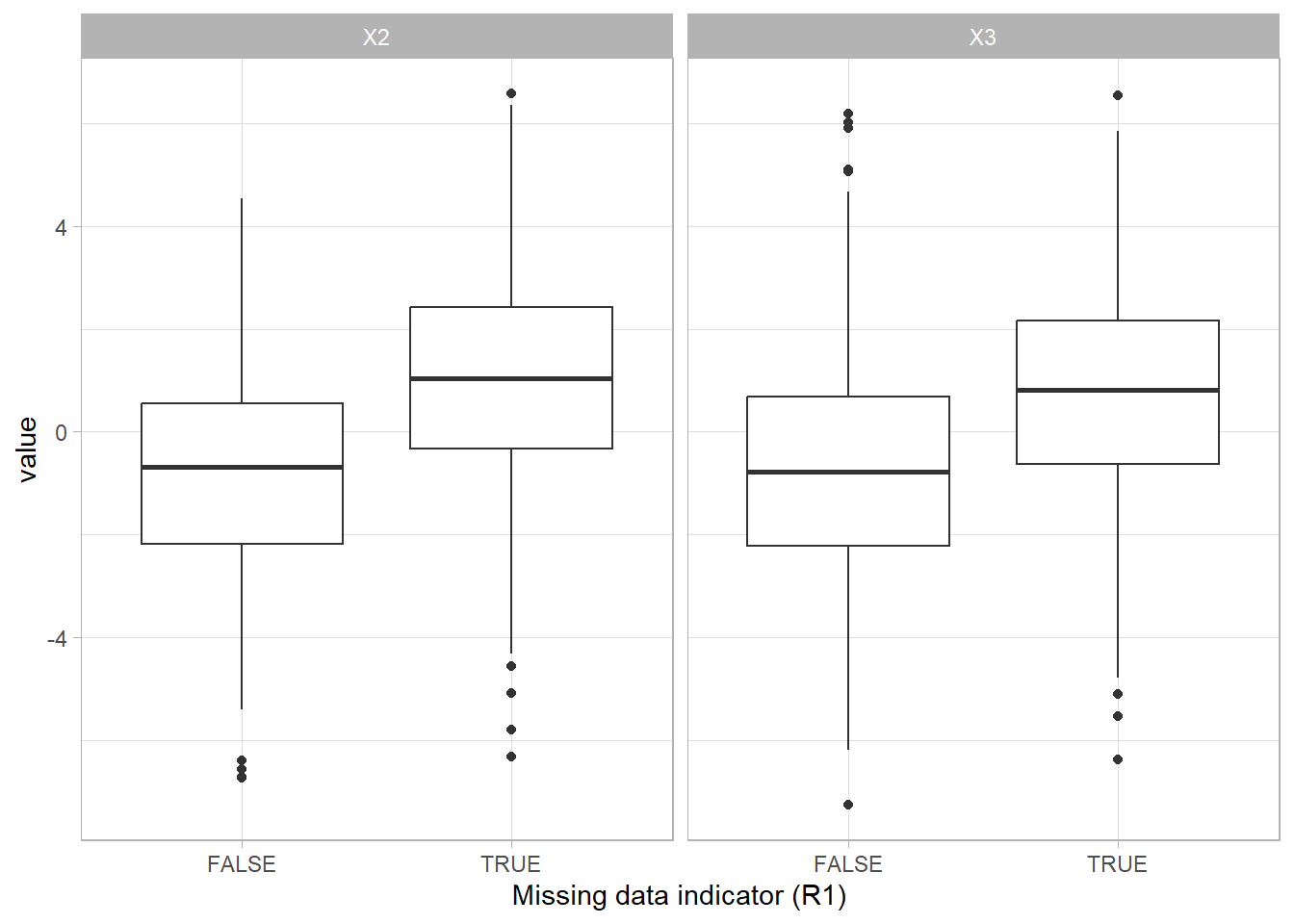
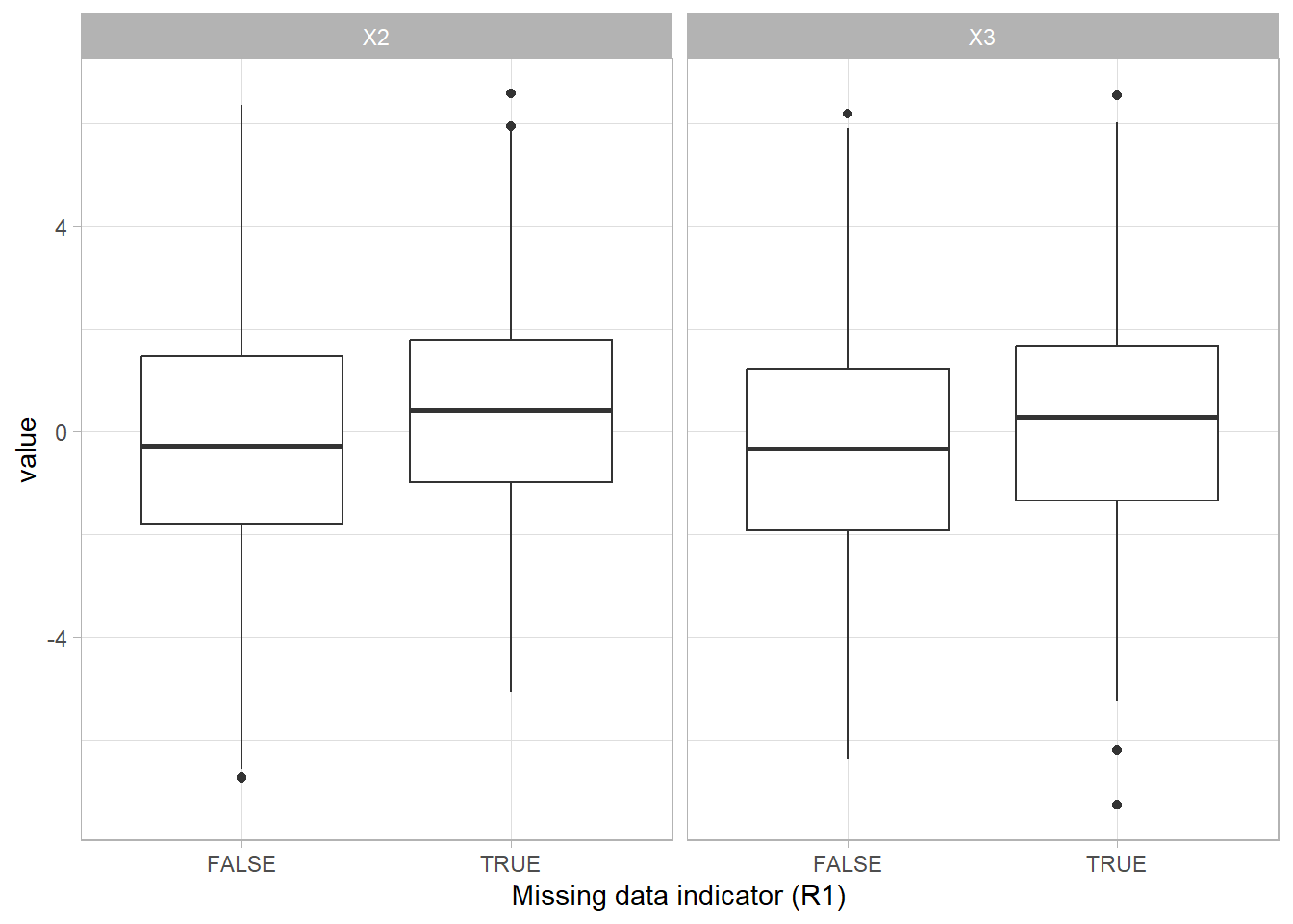
We can create a missing data indicator variable R1 to explore differences between the subjects with missing data and the subjects without missing data.

mar <- mar %>% mutate(R1 = is.na(X1))

The difference between the group with missing values (TRUE) and the group without missing values (FALSE) shows that having missing data is related to the scores on the other variables.

Missing not at random (MNAR)

Data are missing not at random (MNAR) when the missing values on a variable are related to the values of that variable itself, even after controlling for other variables. For example, when data are missing on IQ and only the people with low IQ values have missing observations for this variable. A problem with the MNAR mechanism is that it is impossible to verify that scores are MNAR without knowing the missing values.

Table 5: Description of fully observed data
	vars	n	mean	sd	median	trimmed	mad	min	max	range	skew	kurtosis	se
X1	1	1000	0.00	2.21	0.07	0.02	2.25	-7.42	6.69	14.11	-0.13	-0.13	0.07
X2	2	1000	0.09	2.26	0.14	0.12	2.24	-6.73	6.58	13.31	-0.12	-0.15	0.07
X3	3	1000	-0.03	2.25	0.02	-0.04	2.27	-7.27	6.54	13.81	0.00	-0.22	0.07

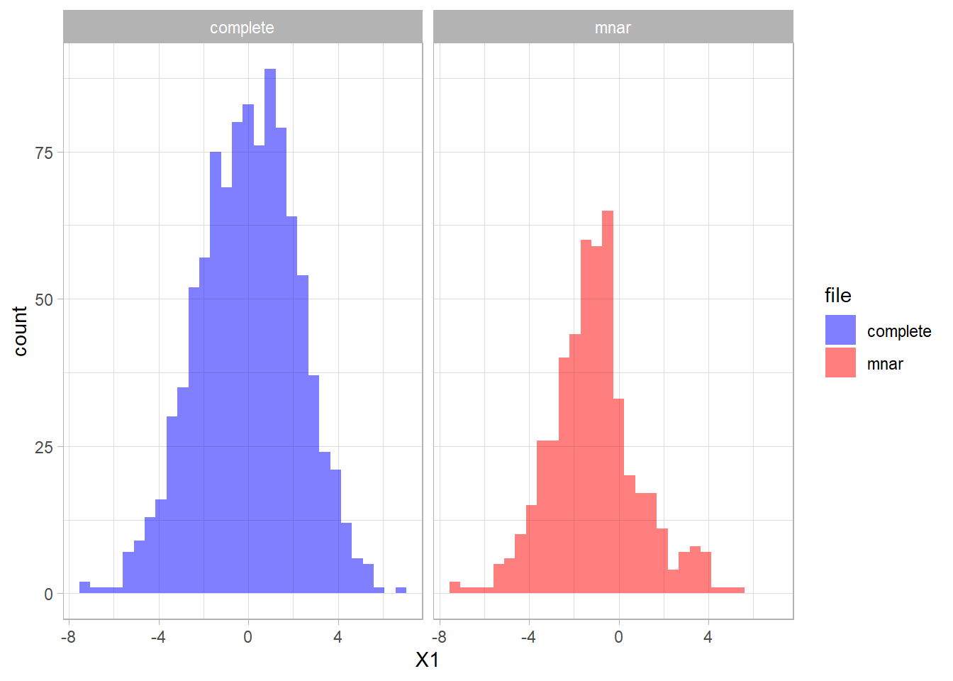
When we create MNAR data for 50% of the subject in variable X1 we see that the statistics for variable X1 have changed:

set.seed(5476)
mnar <- x %>% mutate(rand = runif(1000),
                     X1 = ifelse(X1 > 0 & rand > 0.2, NA, X1), 
                     X1 = ifelse(X1 < 0 & rand > 0.8, NA, X1)) %>%
  select(-rand)

Table 6: Description of MNAR data - 50%
	vars	n	mean	sd	median	trimmed	mad	min	max	range	skew	kurtosis	se
X1	1	488	-1.12	1.96	-1.17	-1.18	1.53	-7.42	5.11	12.53	0.26	0.73	0.09
X2	2	1000	0.09	2.26	0.14	0.12	2.24	-6.73	6.58	13.31	-0.12	-0.15	0.07
X3	3	1000	-0.03	2.25	0.02	-0.04	2.27	-7.27	6.54	13.81	0.00	-0.22	0.07

The distribution of the fully observed version of the variable is depicted in blue and the remaining data due to missings is red. We can compare the two distributions and see that missings occurred mostly in the higher values of X1.

We can create a missing data indicator variable R1 to explore differences between the subjects with missing data and the subjects without missing data.

mnar <- mnar %>% mutate(R1 = is.na(X1))

The difference between the group with missing values (TRUE) and the group without missing values (FALSE) shows that having missing data is related to the scores on the other variables.

Evaluate the missing data mechanism

Any information about the research process can provide valuable information that helps to evaluate and make assumptions about the missing data mechanism. By what is known about the data collection process and the data in general, most researchers have an idea about the reasons for the missing data. It is very important to take this knowledge into account when making an assumption about the missing data mechanism.

Missing data mechanisms

Missing completely at random: missing data is a completely random subsample of the observed data.
Missing at random: probability of missing data is related to other measured variables.
Missing not at random: probability of missing data is related to the missing data itself, and other measured variables.

Testing the mechanisms

The missing data mechanisms are defined by the probability that missing data occur. When this probability is totally not related to other measured variables, we can assume that the remaining sample is a totally random subsample (MCAR).

When other measured variables are related tot the probability of missing data, we can assume that the data are not MCAR. However, we can never definitively rule out MNAR, because we in practice we never know the missing data itself.

Statistical tests

The essence of testing for MCAR is to compare the group with missing data to the group without missing data. We can use simple statistics tests to do this.

Univariate testing

Independent samples t-test to compare for continuous measures
Chi-square test to compare for categorical measures

Multivariate testing

Logistic regression to evaluate multivariately
Little’s MCAR test

T-test to evaluate MCAR

To compare the continuous variables for the group with missing data to the group without missing data, we can use a T-test to compare the means between the groups.

MCAR example

t.test(X2 ~ R1, data = mcar)

## 
##  Welch Two Sample t-test
## 
## data:  X2 by R1
## t = -0.11866, df = 996.42, p-value = 0.9056
## alternative hypothesis: true difference in means between group FALSE and group TRUE is not equal to 0
## 95 percent confidence interval:
##  -0.2970947  0.2632135
## sample estimates:
## mean in group FALSE  mean in group TRUE 
##          0.07756972          0.09451031

MAR example

t.test(X2 ~ R1, data = mar)

## 
##  Welch Two Sample t-test
## 
## data:  X2 by R1
## t = -13.814, df = 994.06, p-value < 2.2e-16
## alternative hypothesis: true difference in means between group FALSE and group TRUE is not equal to 0
## 95 percent confidence interval:
##  -2.064496 -1.550917
## sample estimates:
## mean in group FALSE  mean in group TRUE 
##          -0.7959512           1.0117550

MNAR example

t.test(X2 ~ R1, data = mnar)

## 
##  Welch Two Sample t-test
## 
## data:  X2 by R1
## t = -3.9996, df = 973.87, p-value = 6.824e-05
## alternative hypothesis: true difference in means between group FALSE and group TRUE is not equal to 0
## 95 percent confidence interval:
##  -0.8467042 -0.2893187
## sample estimates:
## mean in group FALSE  mean in group TRUE 
##          -0.2046124           0.3633990

Usually, you do this for all variables in the data that you suspect can be related to the probability of missing data. When there are no significant differences we may assume the data are MCAR. Otherwise, we assume not-MCAR (i.e. MAR or MNAR). Note that we can never truly rule out MNAR.

Chi-square test to evaluate MCAR

To compare the categorical variables for the group with missing data to the group without missing data, we can use a Chi-square test to compare the distribution over the categories between the groups.

MCAR example

mcar <- mcar %>% mutate(X3c = ifelse(X3 > 0, 1, 0))
chisq.test(mcar$R1, mcar$X3c)

## 
##  Pearson's Chi-squared test with Yates' continuity correction
## 
## data:  mcar$R1 and mcar$X3c
## X-squared = 0.062121, df = 1, p-value = 0.8032

MAR example

mar <- mar %>% mutate(X3c = ifelse(X3 > 0, 1, 0))
chisq.test(mar$R1, mar$X3c)

## 
##  Pearson's Chi-squared test with Yates' continuity correction
## 
## data:  mar$R1 and mar$X3c
## X-squared = 80.787, df = 1, p-value < 2.2e-16

MNAR example

mnar <- mar %>% mutate(X3c = ifelse(X3 > 0, 1, 0))
chisq.test(mar$R1, mnar$X3c)

## 
##  Pearson's Chi-squared test with Yates' continuity correction
## 
## data:  mar$R1 and mnar$X3c
## X-squared = 80.787, df = 1, p-value < 2.2e-16

Logistic regression to evaluate MCAR

The probability of missing data can also be investigated in a logistic regression analysis. The missing data indicator is the dependent variable and the other variables that may be related to the probability of missing data are added as the independent variables. Note that when the other variables have missing values as well, a complete-case analysis is used per default.

The results of the logistic regression analysis show if the independent variables relate to the probability of missing data.

MCAR example

glm(R1 ~ X2 + X3, data = mcar) %>%
  summary

## 
## Call:
## glm(formula = R1 ~ X2 + X3, data = mcar)
## 
## Deviance Residuals: 
##     Min       1Q   Median       3Q      Max  
## -0.5489  -0.5094   0.4612   0.4901   0.5299  
## 
## Coefficients:
##              Estimate Std. Error t value Pr(>|t|)    
## (Intercept)  0.509626   0.015841  32.171   <2e-16 ***
## X2           0.001980   0.007142   0.277    0.782    
## X3          -0.006219   0.007148  -0.870    0.384    
## ---
## Signif. codes:  0 '***' 0.001 '**' 0.01 '*' 0.05 '.' 0.1 ' ' 1
## 
## (Dispersion parameter for gaussian family taken to be 0.2504582)
## 
##     Null deviance: 249.90  on 999  degrees of freedom
## Residual deviance: 249.71  on 997  degrees of freedom
## AIC: 1458.4
## 
## Number of Fisher Scoring iterations: 2

MAR example

glm(R1 ~ X2 + X3, data = mar) %>%
  summary

## 
## Call:
## glm(formula = R1 ~ X2 + X3, data = mar)
## 
## Deviance Residuals: 
##      Min        1Q    Median        3Q       Max  
## -1.17785  -0.37994  -0.01758   0.39236   1.20987  
## 
## Coefficients:
##             Estimate Std. Error t value Pr(>|t|)    
## (Intercept) 0.483065   0.013972  34.573   <2e-16 ***
## X2          0.078489   0.006299  12.460   <2e-16 ***
## X3          0.056167   0.006304   8.909   <2e-16 ***
## ---
## Signif. codes:  0 '***' 0.001 '**' 0.01 '*' 0.05 '.' 0.1 ' ' 1
## 
## (Dispersion parameter for gaussian family taken to be 0.1948431)
## 
##     Null deviance: 249.86  on 999  degrees of freedom
## Residual deviance: 194.26  on 997  degrees of freedom
## AIC: 1207.3
## 
## Number of Fisher Scoring iterations: 2

MNAR example

glm(R1 ~ X2 + X3, data = mnar) %>%
  summary

## 
## Call:
## glm(formula = R1 ~ X2 + X3, data = mnar)
## 
## Deviance Residuals: 
##      Min        1Q    Median        3Q       Max  
## -1.17785  -0.37994  -0.01758   0.39236   1.20987  
## 
## Coefficients:
##             Estimate Std. Error t value Pr(>|t|)    
## (Intercept) 0.483065   0.013972  34.573   <2e-16 ***
## X2          0.078489   0.006299  12.460   <2e-16 ***
## X3          0.056167   0.006304   8.909   <2e-16 ***
## ---
## Signif. codes:  0 '***' 0.001 '**' 0.01 '*' 0.05 '.' 0.1 ' ' 1
## 
## (Dispersion parameter for gaussian family taken to be 0.1948431)
## 
##     Null deviance: 249.86  on 999  degrees of freedom
## Residual deviance: 194.26  on 997  degrees of freedom
## AIC: 1207.3
## 
## Number of Fisher Scoring iterations: 2

In the MCAR example we see that both X2 and X3 are not related to the probability of missing data in X1, so we may assume that the missing data in X1 are MCAR. However, in the MAR example, both variables are related tot he probability of missing data in X1, so in that case we can assume that the data are not-MCAR. We cannot rule-out MNAR in this situation, since cannot test the missing values itself.

Little’s MCAR test

Another test that is especially developed by Todd Little, to investigate the MCAR missing data mechanism is Little’s MCAR test. This is a multivariate test, that evaluates the subgroups of the data that share the same missing data pattern. For these subgroups the observed means are compared to the estimated means based on the expectation-maximization algorithm. A chi-square distribution test is used to test the null hypothesis that the data are MCAR. A significant result shows that the data are not-MCAR.

MCAR example

misty::na.test(mcar %>% select(X1:X3))

##  Little's MCAR Test
## 
##      n nIncomp nPattern chi2 df  pval 
##   1000     510        2 0.77  2 0.679

MAR example

misty::na.test(mar %>% select(X1:X3))

##  Little's MCAR Test
## 
##      n nIncomp nPattern   chi2 df  pval 
##   1000     488        2 222.52  2 0.000

MNAR example

misty::na.test(mnar %>% select(X1:X3))

##  Little's MCAR Test
## 
##      n nIncomp nPattern   chi2 df  pval 
##   1000     488        2 222.52  2 0.000

Using Little’s MCAR test does not provide specific information about which variables are related to the probability of missing data. Also, the test assumes multivariate normality and can only be applied to continuous variables. And the MNAR mechanism can never be ruled out, regardless of the result of the test.

Assuming the missing data mechanism

The methods to deal with missing data, implicitly assume a missing data mechanism. The most strict assumption is the MCAR assumption. In practice it is also easiest to deal with MCAR data. Since the data are missing completely at random, we can either just analyze the observed sample only (this will result in unbiased estimates), or use a random imputation method to boost the power the the amount of missing data is too large. In the latter situation, it may be best to use multiple imputation or stochastic regression imputation to retain the covariance structure of the data.

The less strict assumption is the MAR missing data mechanism. Most of the more advanced missing data methods assume this mechanism (e.g. multiple imputation). It is important to make the assumption of the missing data mechanism as plausible as possible. One strategy is to take this into account in the study design. When variables are included that may later explain the missing data, a MAR assumption may become more plausible (as compared to MNAR). These additional variable may also help in dealing with the missing data, because they can be used as auxiliary variables. Auxiliary variables are variables related to the probability of missing data or to the variable with missing data. These variables can be used as predictors in an imputation model or as covariate in a FIML model to improve estimations.

The least strict assumption is the MNAR missing data mechanism. MNAR data are also referred to as non-ignorable, because these cannot be ignored without causing bias in results. MNAR data are more challenging to deal with.

Missing data mechanisms

Missing completely at random (MCAR)

Missing at random (MAR)

Missing not at random (MNAR)

Evaluate the missing data mechanism

Missing data mechanisms

Testing the mechanisms

Statistical tests

T-test to evaluate MCAR

Chi-square test to evaluate MCAR

Logistic regression to evaluate MCAR

Little’s MCAR test

Assuming the missing data mechanism

Iris Eekhout, PhD

Statistician

Related